This is an excerpt from "How Magnetic Bearings Work" document. To read the preceding section click here.
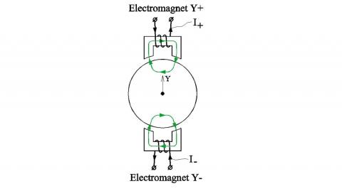
Since the force between an electromagnet and a ferrous object is always an attractive one, the Active Magnetic Bearing shown in Fig. 3 can operate only if the external forces acting on the object (such as the gravity force Fgrav) are directed away from the electromagnet. If the external force can change sign, two electromagnets located on the opposite sides of the object along the force line must be used as shown in Fig. 4. For example, if the external force is applied in the positive Y direction, the bottom electromagnet in Fig. 4 can be energized to counteract that force and keep the object in place. Alternatively, if the external force is applied in the negative Y direction, the top electromagnet can be energized to counteract it.
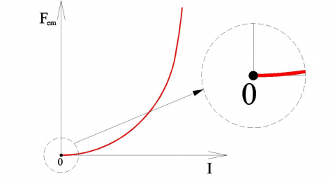
In practical applications, the external force acting on an object (the rotor of a machine supported by a magnetic bearing) will vary with time or reverses sign. This makes the current control in of the electromagnetic much more difficult than when the external force is constant (such as the gravity force in Fig. 3). To understand these complications, we need to look at how the force exerted by the electromagnet on the object depends on the current in the electromagnet. This dependence is quadratic in nature: Fem~I2 . Fig. 5 shows an example of Fem vs I curve. Note that the slope of this curve is not constant and changes with the current (force). Particularly important is that when we try to generate a small force close to zero, the force doesn’t respond much to changes in the current. This makes choosing the right current to offset an external force and stably levitate an object at the desired position difficult.
FIG. 4
FIG. 5
A common method used to avoid complications with non-linearity of the Fem vs I curve is to pre-energize both electromagnets Y+ and Y- in Fig. 4 with the same constant current I0 called bias current. If the object in Fig. 4 is centered between two identical electromagnets and both are energized with the same current, the net pull force on the object would be zero (the bottom electromagnet would pull the object down with exactly the same force as the top electromagnet would pull it up). Therefore, with bias current I0 alone there is no net electromagnetic force on a centered object.
In order to produce a net force, an additional current, called control current Ic, is injected into both electromagnets in such a way that if it adds to the bias current in one coil, it subtracts from it in another coil. For example, in order to produce a force in the positive Y direction, the control current Ic has to be added to the bias current I0 in the top electromagnet and subtracted from it in the bottom electromagnet. Then the force produced by the top electromagnet would be
F+~(I0 + Ic)2 (1)
and the force produced by the bottom electromagnet would be
F_~(I0 - Ic)2. (2)
The net force exerted on the object would be
F = F+ – F _ ~(I0 + Ic)2 – (I0 - Ic)2 = 2I0Ic. (3)
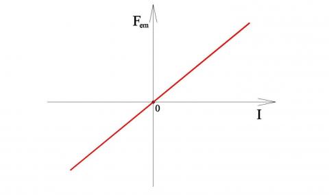
If the bias current I0 is kept constant and the object is kept at the center between two electromagnets, the electromagnetic force exerted on the object would be simply a linear function of the control current (Fig. 6). Reversing sign of the control current will reverse the sign of the force.
FIG. 6
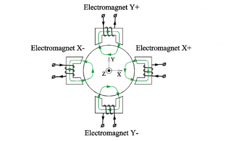
The object position can be controlled along two axes - X and Y, if two more electromagnets are added as shown in Fig. 7. The structure shown in Fig. 7 represents the typical basic radial active magnetic bearing design employed by most magnetic bearing companies (Calnetix utilizes a different approach as will be discussed later). The only difference is that in practical designs individual electromagnets are often linked together by a common ferrous path and there might be different poles arrangements.