PM Bias, Homopolar Magnetic Bearings

This is an excerpt from "How Magnetic Bearings Work" document. To read the preceding section click here. 

Calnetix has pioneered commercial use and holds several key patents on another type of radial active magnetic bearing – the homopolar, PM-biased active magnetic bearing. The basic structure of such a radial active magnetic bearing is shown in Fig. 9, a 3D illustration in Fig. 10 and the operational principle is explained in Fig. 11.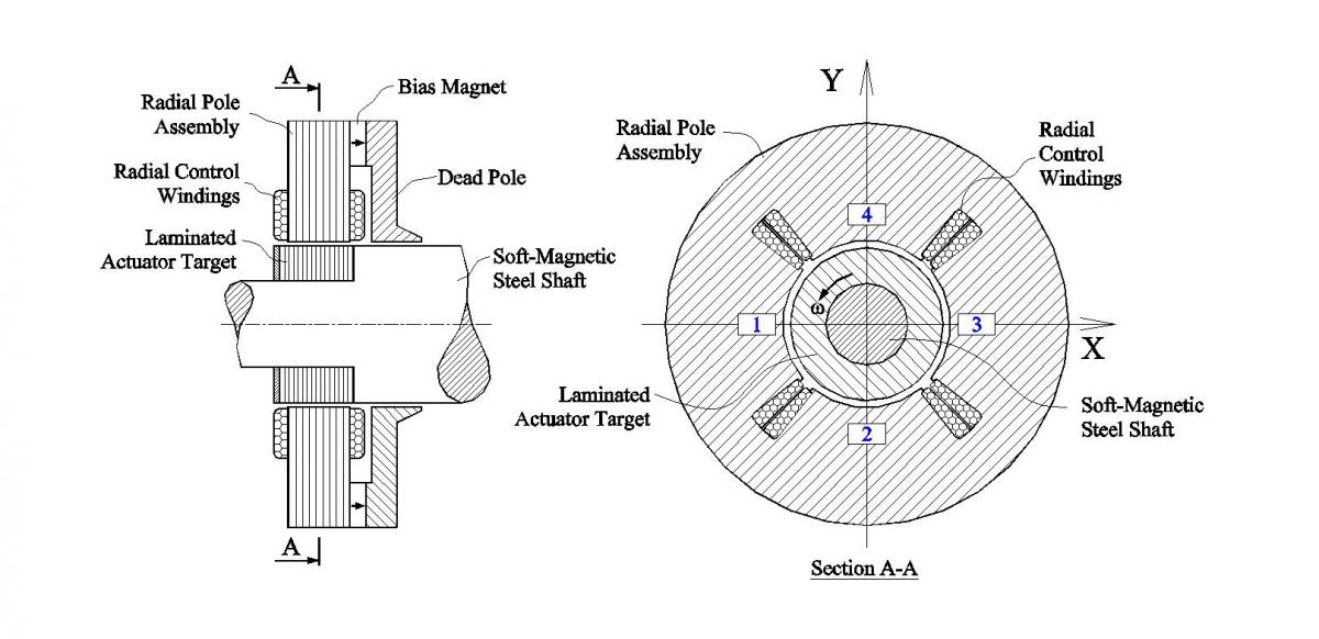                                                                                                       FIG. 9

 

                                                                                                    FIG. 10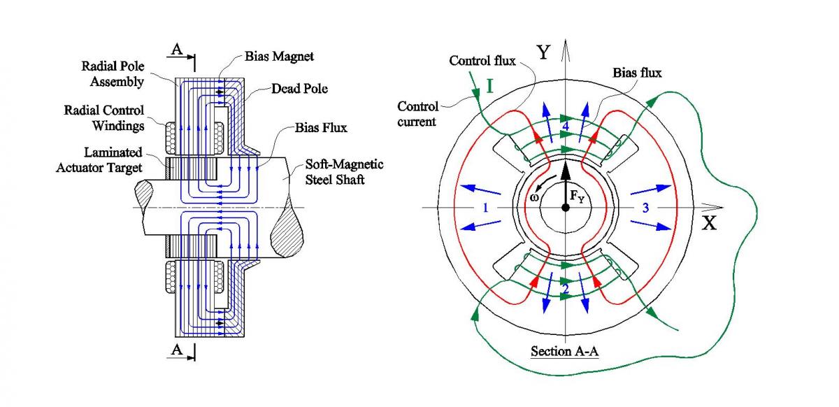                                                                                                    FIG. 11

 

To better understand the operation of this type of radial magnetic bearing, we need to note that the magnetic field in the air gap between the electromagnet poles and the rotor is proportional to the control current. Thus there is a bias magnetic field component B0 that is proportional to I0. Similarly, there is a control magnetic field component Bc that is proportional to Ic. Then, equation (3) can be re-written in terms of magnetic fields (magnetic flux densities) instead of currents:

F~2B0Bc~2B0Ic  (5)

One important difference between the radial active magnetic bearing shown in Figs. 9 through 11 and the one shown in Figs. 7 and 8 is that the bias magnetic field B0 in Figs. 9 - 11 is generated by permanent magnets rather than currents in coils. A critical advantage of permanent magnets is that they produce the bias magnetic field without consuming power, and even more importantly, without generating heat. This translates into a smaller size for the PM bias active magnetic bearing compared to an equivalent EM biased active magnetic bearing. The explanation is as follows.

When a certain magnetic field is generated by a coil, the resistive heat generated by this coil in the process depends inversely on the amount of a conductive material (typically copper) in the coil: more copper means less heat. Because the coil temperature rise and subsequent heat generation must be limited, the size of a typical electric coil needed to generate a certain magnetic field in an active magnetic bearing is several times bigger than a modern rare-earth magnet needed to generate the same field.

While it is possible to use a dedicated coil to generate the bias magnetic fields in EM biased active magnetic bearings, in most commercial implementations a single coil accommodates both the bias and control currents. The advantages of this approach are fewer terminal wires, less complexity and less cost, while the disadvantage is a lower dynamic force capacity due to increased inductance of the combined bias/control coil. In any case, either the net size of both dedicated bias and control coils or a the size of a combined bias/control coil in and EM biased active magnetic bearing would be significantly larger than the combined size of a permanent magnet and a control coil in a PM-biased active magnetic bearing.  A smaller magnetic bearing normally leads to better rotordynamic performance of a machine and more robust operation.

In Calnetix Radial AMBs, the permanent magnet generating the bias magnetic field is sandwiched axially between a radial pole assembly and so called "dead" pole as shown in Figs. 9 through 11. The bias magnetic field generated by the magnets is delivered by the "dead" pole to a soft-magnetic shaft, which further transfers the field to a laminated actuator target. The field exits the target radially, crosses radial air gap, enters the radial pole assembly and travels within it towards the magnet to complete the loop.

The radial pole assembly has two pairs of diametrically opposite magnetic poles with electrical windings around them. The electrical windings associated with each pole pair are connected in series so that they produce magnetic fields in the same direction along the pole axis.

Fig. 11 illustrates generation of a radial force along the vertical Y axis as an example. When the coils wound around poles 2 and 4 are energized with a current I as shown in Fig. 11, they produce a control magnetic flux that adds to the bias flux in the top air gap under the pole #4 and subtracts from it in the bottom air gap under the pole #2. As a result, the net magnetic flux density becomes larger in the top air gap, and the magnetic force pulling the rotor toward the pole #4 (up) becomes larger than the force pulling it towards the pole #2 (down). Thus applying a control current to coils #2 and #4 results in a net magnetic force directed upwards (positive Y direction). Reversing the current reverses the direction of the force. Applying a current in a similar manner to coils #1 and # 3 will produce a force in the X directions and a combination of two currents allows generating a force in any direction in the radial plane.

A very important advantage of the bearing shown in Figs. 9-11 over the bearing shown in Figs. 7-8 is that the bias magnetic polarity is uniform around the circumference of the rotor. For example, in Figs. 9-11 each of the control poles #1 through #4 has "South" polarity and the entire ID of the dead pole has "North" polarity. Therefore, almost no bias flux will be expelled from the rotor due to eddy currents induced when the rotor spins as opposed to the design shown in Figs. 7-8 (a small portion of the bias flux will be expelled because of discontinuities between active poles 1-4). If we were only concerned about the bias field, the actuator target on the rotor would not even have to be laminated.

When the bearing shown in Figs. 9-11 generates a radial force, such as FY force in Fig. 11, however, the control component of the magnetic field will be non-uniform around the rotor and it will tend to be expelled by the eddy currents. Even if we lose only Bc component in equation (5), however, we still lose the load capacity. Therefore, the actuator target in the design per Figs. 9-11 still has to be laminated.

Important advantages of the design shown in Figs. 9-11 over the design shown in Figs. 7-8 at speed is that

a.) There is no loss of B0. Therefore, if the same laminations as in heteropolar bearings are used, and even if we assume that Bc is the same as in heteropolar bearings, the load capacity would already be retained better at speed than in heteropolar bearings. (In reality Bc in homopolar bearings will also be higher at speed than in heteropolar ones as explained below in item b.).

b.) The frequency of the control magnetic field variations that the rotor sees at speed are at least two times lower in the design per Figs. 9-11 than in the design per Figs. 7-8. According to eq. (4), this means that either Bc will be retained better at speed, or thicker (cheaper) laminations can be used.

Both items a.) and b.) above lead to better retention of the load capacity in homopolar bearings at speed (provided that the same lamination thicknesses are used).

Click here to read the next section.